
Excel’s worksheet function list doesn't include QUERY. Google documents QUERY as a Google Sheets function.
QUERY syntax and its Excel alternatives
Google Sheets QUERY takes 3 arguments:
=QUERY(data, query, [headers])
datais the source range.queryis a text string containing selection, filtering, grouping, or sorting instructions.[headers]identifies the number of header rows in the source.
The closest Excel alternatives are:
| QUERY clause | Purpose | Excel alternative |
|---|---|---|
select | Choose returned columns | CHOOSECOLS or explicit references |
where | Include records meeting specified conditions | FILTER |
group by | Summarize records by one or more dimensions | UNIQUE with SUMIFS, or a PivotTable |
order by | Sort the result | SORT or SORTBY |
limit | Return a specified number of rows | TAKE, where available |
label | Set output headings | Headings entered in worksheet cells |
These tools don't provide exact feature parity with QUERY. Instead, they reproduce common selection, filtering, sorting, and aggregation tasks through a different formula structure.
For native QUERY examples, see how to use QUERY in Google Sheets.
Excel requirements for these formulas
The procedures below require an Excel for Microsoft 365 installation that supports dynamic arrays, LET, FILTER, SORT, CHOOSECOLS, and UNIQUE. Microsoft lists compatible editions under “Applies To” in its documentation for FILTER, SORT, and CHOOSECOLS.
You can test compatibility without relying on locale-specific array constants:
- In a blank worksheet, enter
1,2, and3inA1:C1. - Enter this formula in
A2:
=CHOOSECOLS(A1:C1,1,3)
A compatible installation spills 1 into A2 and 3 into B2. If Excel returns #NAME?, use the PivotTable or Power Query methods later in this article. You can also build the output with helper columns and conventional copied formulas.
The examples use commas as function argument separators. Some regional settings require semicolons.
Reproduce the native Google Sheets example
Use the synthetic Spreadsheet formula and cleanup practice workbook:
Use the Google Sheets copy for native QUERY formulas. The XLSX companion provides the source data, guidance, and a portable SUM(F160:H160) formula. It doesn't contain native Google QUERY outputs.
1. Review the source range
Start with Transactions!A1:F13. Row 1 contains the headers, and the examples use:
- Column A: Date
- Column B: Category
- Column D: Amount
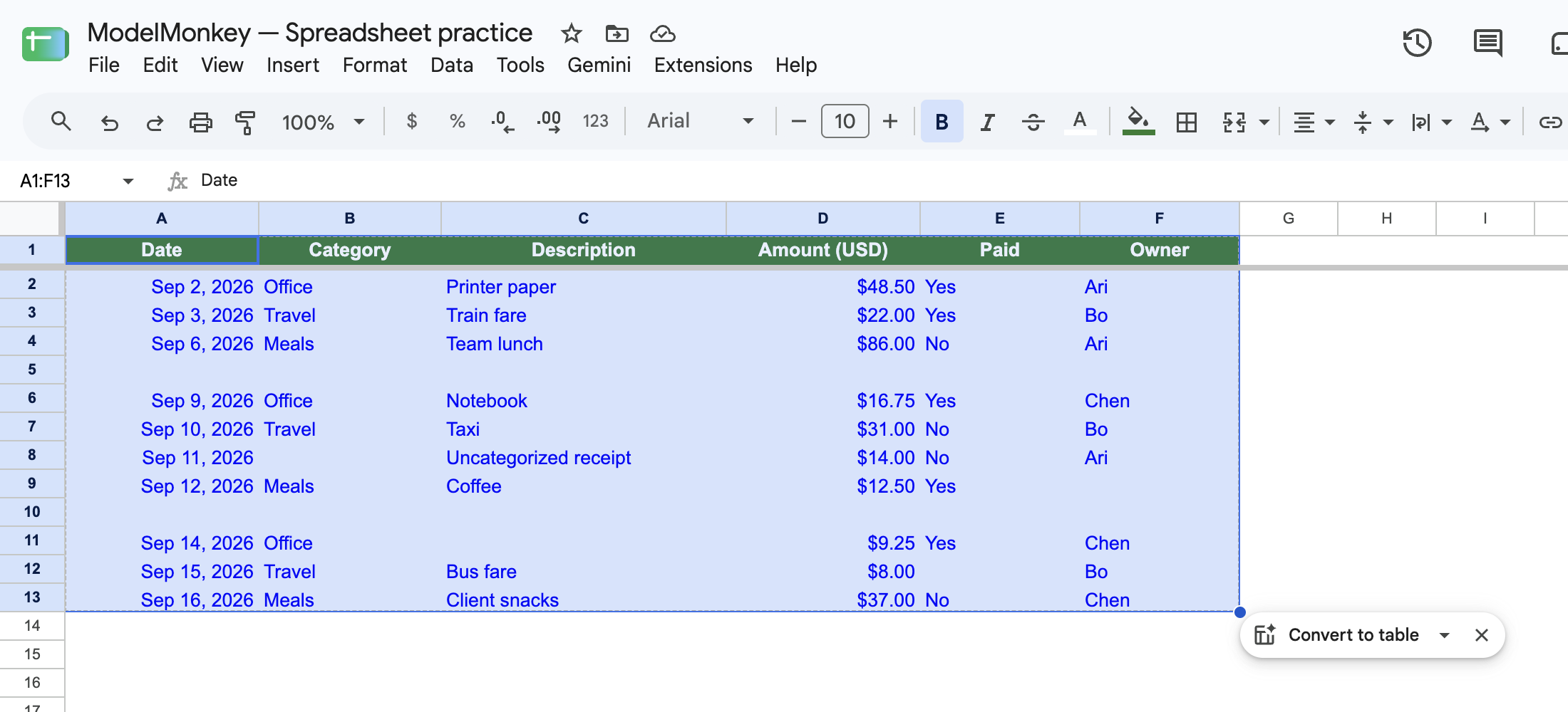
Actual Google Sheets screenshot of the restored synthetic example.
Rows 5 and 10 are wholly blank. However, the records in A8:F9 and A11:F12 are only partial, so don't delete them solely because some fields are empty.
Delete a complete row only after confirming that the entire row is blank. Deleting one blank cell and shifting the remaining cells can separate fields from their original records.
2. Filter for populated Dates with QUERY
In the native Google Sheets copy, Practice!A18 contains:
=QUERY(Transactions!A1:F13,"select * where A is not null",1)
This formula:
- Returns every source column with
select *. - Keeps records whose Date isn't null.
- Treats the first source row as a header because the final argument is
1.
The recorded result in Practice!A18:F28 contains the header plus 10 dated records. It excludes the 2 wholly blank rows while retaining dated partial records.
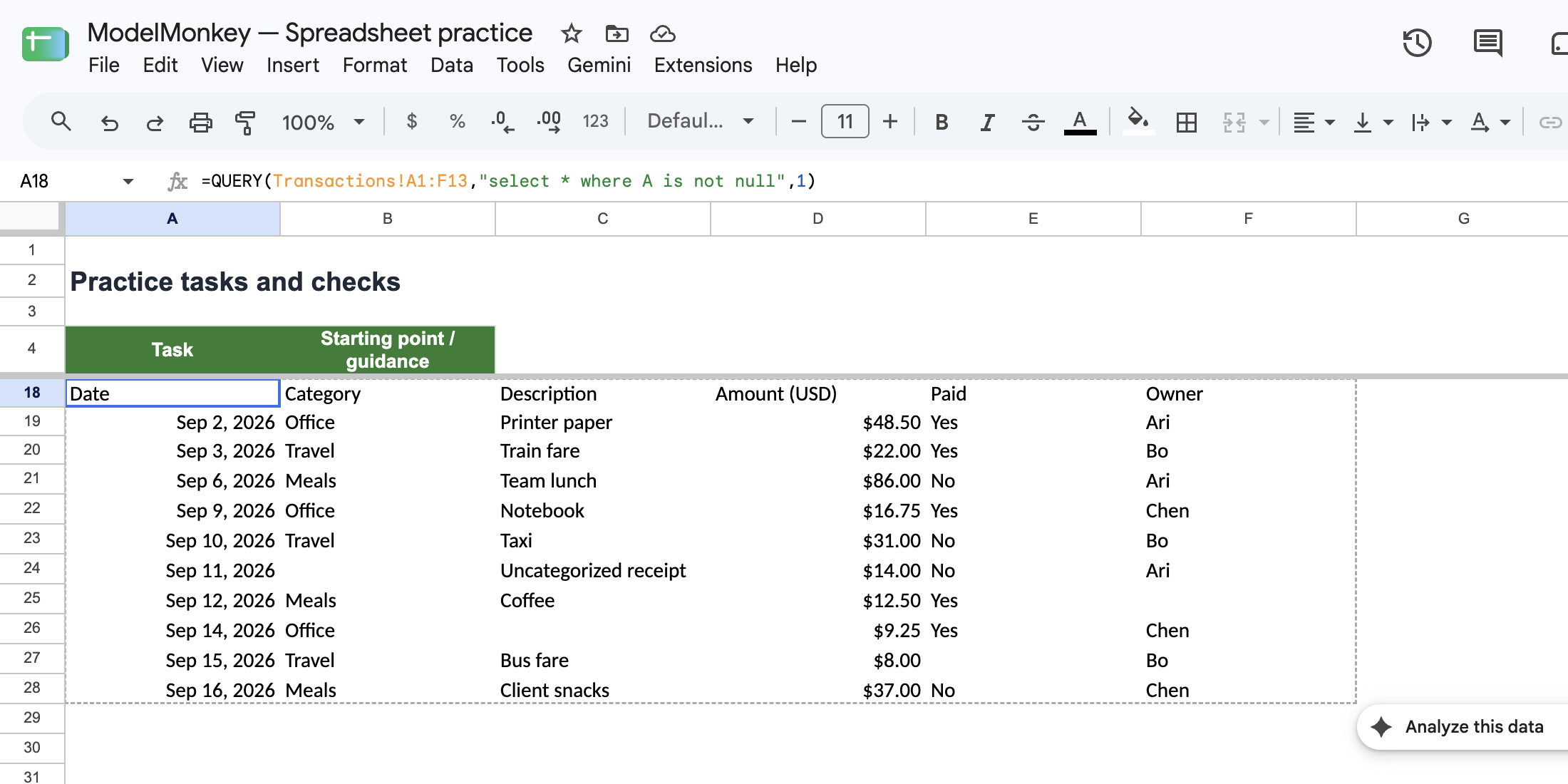
Native QUERY excludes wholly blank rows and keeps incomplete records for review.
This condition tests only Date. It doesn't validate Category, Amount, or other required fields. Whitespace-only text may also pass a basic nonblank check, so it requires separate cleanup.
Practice!A32 contains a separate category-grouping QUERY. Its formula and returned categories weren't included in the recorded execution evidence, so that output isn't used as a control here.
3. Establish the Office control total
Practice!B15 contains:
=SUMIFS(
  Transactions!$D$2:$D$13,
  Transactions!$B$2:$B$13,
  "Office"
)
The recorded result is 74.5. Because the fixture doesn't define a currency, this is an amount rather than a dollar value.
Before replacing any formula, copy B15 and paste its value into an empty cell or duplicate tab. Doing so preserves 74.5 as a static reconciliation control.
Recreate filtering, selection, and sorting in Excel
The following Excel formulas are proposed translations. Recorded execution covers the native Google Sheets results, not an Excel run.
Add a sheet named Excel Alternatives, then enter these headings:
| Cell | Value |
|---|---|
A1 | Date |
B1 | Category |
C1 | Amount |
Enter this formula in A2:
=LET(
  data,Transactions!A2:F13,
  keep,Transactions!A2:A13<>"",
  IF(
    SUM(--keep)=0,
    "No matching rows",
    SORT(
      CHOOSECOLS(FILTER(data,keep),1,2,4),
      1,
      1
    )
  )
)
The formula performs 4 operations:
FILTERkeeps records with a nonblank Date.CHOOSECOLSreturns Date, Category, and Amount from source columns 1, 2, and 4.SORTorders the result by Date ascending.IFreturns one cell containingNo matching rowswhen no Dates are populated.
The expected output is 10 rows by 3 columns, matching the population returned by the native QUERY. Keep the cells below and beside A2 empty so the array can spill.
If Excel returns #SPILL!, inspect the output area for occupied or merged cells. See Excel spill error causes for other common blockers.
Like the native QUERY, this formula tests only Date. It doesn't confirm that each Date is valid or that every other field is complete.
Recreate QUERY GROUP BY with UNIQUE and SUMIFS
For a consistent category summary, apply the same criteria throughout: include records with both a populated Date and Category.
First, create a dated Office control. Enter Dated Office Control in Excel Alternatives!E1, then place this formula in E2:
=SUMIFS(
  Transactions!$D$2:$D$13,
  Transactions!$B$2:$B$13,
  "Office",
  Transactions!$A$2:$A$13,
  "<>"
)
For the supplied fixture, the expected result remains:
74.5
This result agrees with the recorded category-only control in Practice!B15 because the fixture’s only blank-Date rows are wholly blank. In another workbook, a row containing Office but no Date would make the category-only and dated controls differ.
Next, enter Category in G1 and Total Amount in H1.
In G2, enter:
=SORT(
  UNIQUE(
    FILTER(
      Transactions!B2:B13,
      (Transactions!A2:A13<>"")*
      (Transactions!B2:B13<>"")
    )
  )
)
In H2, enter:
=SUMIFS(
  Transactions!$D$2:$D$13,
  Transactions!$B$2:$B$13,
  G2#,
  Transactions!$A$2:$A$13,
  "<>"
)
G2# refers to the complete category list spilled from G2. For each category, SUMIFS returns one total while applying the same nonblank-Date criterion used to create the list.
Microsoft documents UNIQUE and SUMIFS.
To reconcile the results, enter Office Variance in J1 and this formula in J2:
=SUMIFS(H2#,G2#,"Office")-$E$2
The expected result is 0. A zero variance confirms that the grouped Office amount agrees with the dated Office control for this value. It doesn't prove that both outputs contain identical underlying records, since different or offsetting items could produce the same total.
A nonzero result identifies a reconciliation difference, but it doesn't reveal the cause by itself.
The proposed reconciliation is:
| Control | Expected result |
|---|---|
Filtered records in A2# | 10 rows |
Dated Office control in E2 | 74.5 |
| Office amount in grouped output | 74.5 |
Office variance in J2 | 0 |
If no records contain both a Date and Category, G2 returns #CALC!. Treat that result as an exception, not a valid zero total.
Check Amount before relying on grouped totals
A nonblank-Date filter doesn't confirm that Amount contains valid numbers. In a duplicate workbook, add a sheet named Checks. Enter Invalid_Amount_Count in Checks!A2 and this formula in Checks!B2:
=SUMPRODUCT(
  --(Transactions!A2:A13<>""),
  --(Transactions!B2:B13<>""),
  --(ISNUMBER(Transactions!D2:D13)=FALSE)
)
This control counts records where all 3 conditions apply:
- Date is populated.
- Category is populated.
- Amount isn't numeric.
A result of 0 is the pass condition for that defined population. Numeric zero passes because ISNUMBER(0) is true. Negative numeric amounts also pass the type test, although their business validity depends on the workbook’s accounting rules.
A blank-category record isn't counted, so review those records separately. An Excel error value in Amount causes ISNUMBER to return false and is therefore counted as invalid when Date and Category are populated.
Errors in the Date or Category range behave differently. They can propagate through the corresponding comparison and cause the control formula itself to return an error. Correct or isolate source errors before relying on the count.
Use a fresh copy for each independent check:
| Source condition | Expected treatment |
|---|---|
| Wholly blank row | Excluded because Date is blank |
| Dated partial record | Retained for review |
| Numeric zero in Amount | Retained and contributes zero |
| Blank, text, or error Amount with Date and Category populated | Flagged by the numeric control |
| Blank Category with an invalid Amount | Not flagged by this control |
| Error in Date or Category | May cause the control formula to return an error |
| Duplicate transaction | Counted again |
| Date containing only spaces | May pass the nonblank test and requires cleanup |
| Every Date cleared | Excel Alternatives!A2 returns one No matching rows cell |
These formulas don't identify duplicates. If duplicates aren't valid, define a transaction key and add a separate duplicate control.
Use a PivotTable for an interactive summary
A PivotTable works well when you need to rearrange dimensions, apply report filters, or inspect grouped totals without maintaining a formula chain.
Using the same fixture:
- Select
Transactions!A1:F13and insert a PivotTable. - Place Category in Rows.
- Place Amount in Values.
- Confirm that Amount is summarized by Sum, not Count.
- Place Date in Filters and exclude blank Dates.
- Exclude blank Categories to match the
G2:H2formula population. If you retain them for review, reconcile that group separately. - Reconcile the Office amount to
74.5.
Apply the Date exclusion inside the PivotTable. Hiding or filtering worksheet rows doesn't necessarily change the PivotTable’s source population.
Microsoft provides instructions for creating a PivotTable. After creating or refreshing the PivotTable, investigate any difference from the formula control instead of assuming either output is correct.
Use Power Query for repeatable transformations
For repeatable importing, data-type assignment, filtering, merging, or grouping, use Power Query before loading results into Excel.
To create a row-level output:
- Select
Transactions!A1:F13. - Choose Data > From Table/Range and confirm that the first row contains headers.
- Assign an appropriate Date type to Date and a numeric type to Amount.
- Inspect type errors instead of removing them without review.
- Filter Date to exclude null or blank records.
- Keep Date, Category, and Amount.
- Sort Date ascending.
- Close and load the result into a worksheet.
The expected row-count control is 10 records.
For a grouped summary, follow the same process, then:
- Filter Category to exclude null or blank values so the population matches
G2:H2. - Group by Category.
- Sum Amount.
- Close and load the result.
- Reconcile Office to
74.5.
If you retain a blank-category group, present it as a separate exception. Don't include it in a comparison with formulas that exclude blank Categories.
Power Query uses its own editor and M language. It doesn't make Google Sheets QUERY syntax valid in an Excel worksheet cell.
Check the open-ended Google Sheets range
The native workbook also demonstrates an open-ended row reference.
Practice!F160:H160 contains:
2 | 3 | 5
Native Practice!F161 contains:
=SUM(F160:160)
The recorded result is 10. The range starts at column F and continues through the last column in row 160, so it includes F160, G160, and H160.
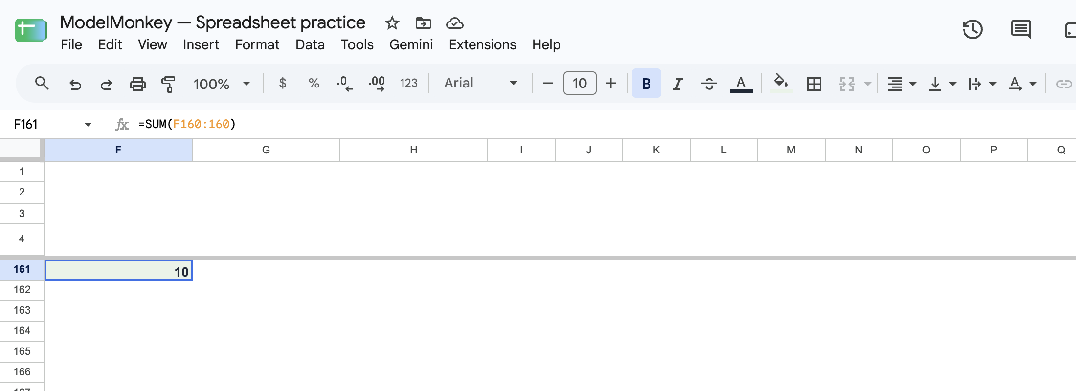
Native Google Sheets accepts this open-ended row range; the Excel download uses F160:H160.
For portability, the XLSX companion uses:
=SUM(F160:H160)
That explicit range produces the same total from the 3 supplied inputs.
Where ModelMonkey fits
ModelMonkey is an AI assistant for spreadsheet work in Google Sheets and Excel. It can inspect workbook context and help read ranges, analyze and organize spreadsheet content, clean data, and propose formula or worksheet changes.
For this workbook, you could ask:
Read Transactions!A1:F13. Help me exclude blank Dates, retain dated partial records for review, select Date, Category, and Amount, group Amount by Category, and reconcile Office to the 74.5 control in Practice!B15.
Check the proposed output against the 10 dated records, the Amount-validity control, and the Office total. When the workflow presents a preview, review the proposed changes before proceeding. Spreadsheet assistance doesn't guarantee that every formula or edit is correct.
Use ModelMonkey to translate a QUERY task for your workbook.